Unit 3
1) Why is deep learning important? Explain with real-world examples.
Why Is Deep Learning Important?
Deep learning is crucial because it allows computers to learn complex patterns from vast and varied data without human-crafted rules. This has led to remarkably accurate and intelligent systems in fields where traditional methods often fall short.
Key Reasons for Its Importance
- Handles Complex Data: Deep learning can learn patterns from unstructured data like images, sound, and human language, automating tasks that were once considered uniquely human.
- Continual Improvement: With more data and computing power, deep learning systems keep improving and adapting without manual intervention.
- Feature Extraction: Instead of relying on human experts to define useful features, deep neural networks discover them automatically, improving accuracy and efficiency.
Real-World Examples of Deep Learning Impact
-
Image Recognition and Computer Vision:
- Powers facial recognition in phones, automatic photo tagging, and even autonomous vehicles that can detect pedestrians, traffic signs, and obstacles.
- Medical imaging tools use deep learning to spot early signs of diseases like cancer in MRI and X-ray scans, sometimes surpassing human experts.
-
Natural Language Processing (NLP):
- Virtual assistants like Siri and Alexa understand and respond to voice commands, chatbots provide customer support, and systems summarize long texts into concise insights.
- Translation apps break language barriers in real time.
-
Speech Recognition:
- Voice typing, real-time transcription in meetings, and smart home control are possible due to deep learning models that convert speech to text accurately, even across accents and in noisy environments.
-
Recommendation Systems:
- Streaming services like Netflix and YouTube suggest content tailored to each user, while e-commerce sites recommend products based on browsing and buying patterns.
-
Healthcare and Drug Discovery:
- AI systems assist doctors in diagnosing diseases, propose effective drug combinations, and accelerate drug discovery, cutting costs and saving lives.
-
Cybersecurity and Fraud Detection:
- Deep learning models flag suspicious activities in banking and online transactions, protecting users from fraud by learning subtle, complex patterns.
-
Smart Cities and Industrial Automation:
- Traffic signals are managed dynamically to reduce jams, and industrial robots automate warehouse work and precision manufacturing.
Summary
Deep learning is important because it powers the technology behind medical breakthroughs, safer transportation, smarter recommendations, robust language tools, and greater automation. Its ability to learn directly from raw data keeps unlocking new possibilities in science, business, and daily life.
2) Differentiate between structured, unstructured, and semi-structured data with examples.
Difference Between Structured, Semi-Structured, and Unstructured Data
Let’s break down the three major data types with definitions and real-world examples:
1. Structured Data
- Definition: Highly organized data with a fixed schema—fits neatly into rows and columns of tables (often managed by relational databases).
- Storage: Databases like SQL, Excel sheets.
- Examples:
- Customer records: Name, Age, Phone Number
- Bank transactions table
- Inventory spreadsheets
- Features: Easy to search, query, analyze; less flexible and harder to scale.
2. Semi-Structured Data
- Definition: Data that is not stored in rigid tables but still has some organization (often via tags or keys); there is no fixed schema, but structural elements exist.
- Storage: NoSQL databases, XML, JSON files.
- Examples:
- XML or JSON documents (e.g., data exported from an app)
- Emails with metadata (subject, timestamp—structured; body text—less structured)
- Digital photos with EXIF metadata (image content is unstructured, but tags like date/time/geotag add structure)
- Features: More flexible than structured data, easier to scale, but harder to analyze than truly structured data; sits between structured and unstructured forms.
3. Unstructured Data
- Definition: Data with no predefined organization or model—cannot be stored as rows/columns; often qualitative and rich in information.
- Storage: Data lakes, filesystems.
- Examples:
- Text documents, social media posts
- Images, videos, audio files
- PDF documents, Word files, media logs
- Features: Most flexible and scalable; hard to query or analyze directly; often requires advanced processing tools like natural language processing or image recognition.
Summary Table
| Type | Structure Level | Storage | Example |
|---|---|---|---|
| Structured | Fixed, rigid | SQL, Spreadsheets | Employee DB table |
| Semi-Structured | Partial, flexible | JSON, XML, NoSQL | JSON blog data, emails |
| Unstructured | None | Data lakes, filesystem | Tweets, videos, PDFs |
In practice: Most organizations work with all three, often combining survey results (structured), customer emails (semi-structured), and reviews or photos (unstructured) for richer analytics.
3) Draw and explain the architecture of a Convolutional Neural Network (CNN).
Architecture of a Convolutional Neural Network (CNN)
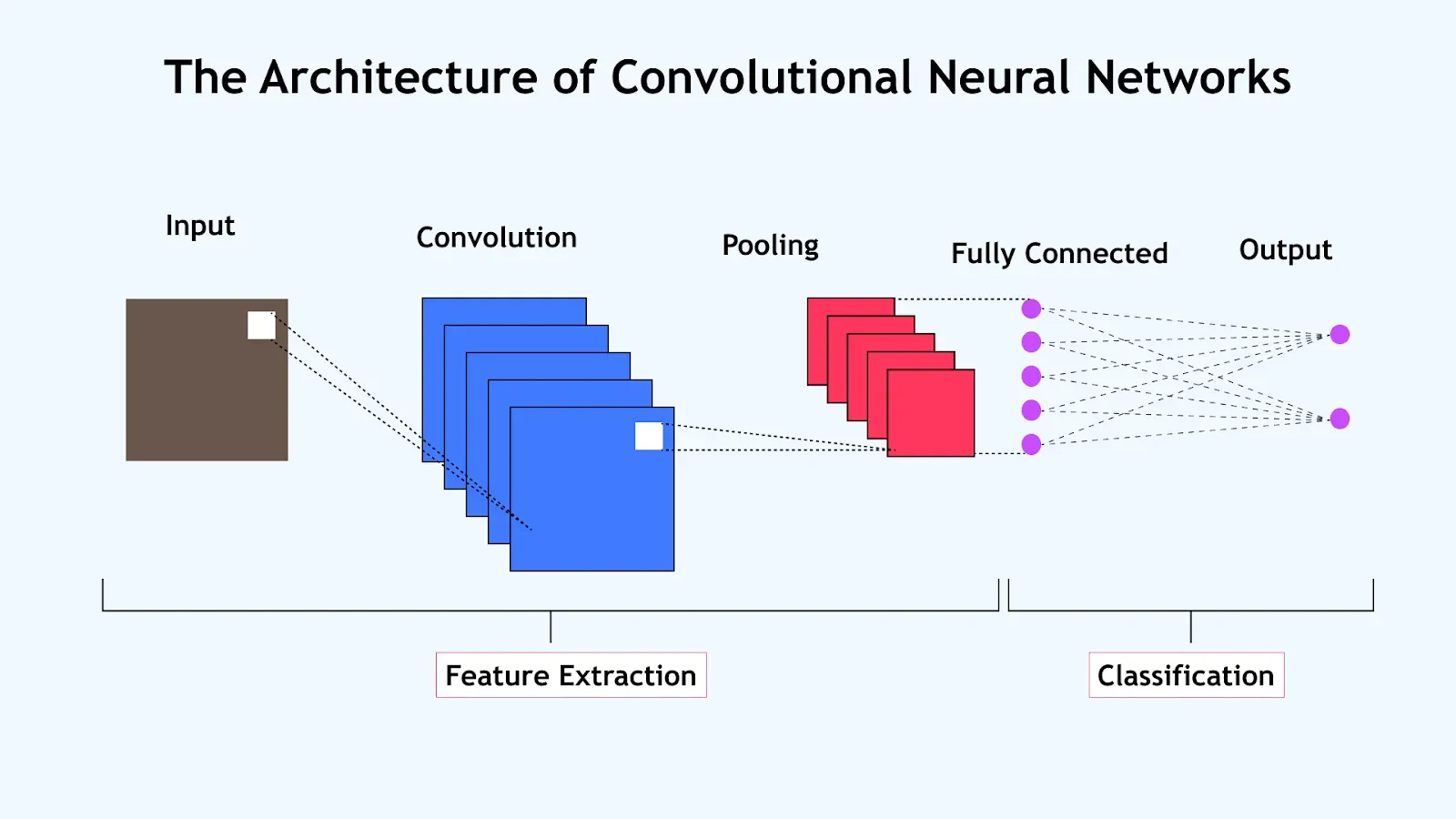
A Convolutional Neural Network (CNN) is a specialized type of neural network particularly effective for processing image and spatial data. CNNs automatically learn spatial hierarchies of features by using different kinds of layers stacked together in a specific order.
1. Input Layer
- Receives the raw data (such as an image). Each pixel forms part of the input vector. For color images, inputs span width, height, and depth (channels).
2. Convolutional Layers
- Apply several small filters (kernels) that slide over the input to extract low- to high-level features (edges, textures, shapes).
- Each filter produces a feature map: an array highlighting where a specific pattern appears in the input.
- These filters are learned automatically during training, allowing the network to detect ever more complex features as you go deeper.
3. Activation Functions
- After each convolution, an activation function (most commonly ReLU: f(x) = max(0, x)) introduces non-linearity, helping the network learn complex relationships.
4. Pooling Layers
- Reduce the spatial dimensions (width and height) of the feature maps, keeping the most important information while lowering computation.
- Max pooling is common: it selects the maximum value from each patch.
- Helps achieve translation invariance and reduces overfitting.
5. (Optional) Normalization & Dropout Layers
- Normalization layers: Standardize activations to improve training stability (e.g., batch normalization).
- Dropout layers: Randomly ignore some neurons during training to reduce overfitting.
6. Fully Connected (Dense) Layers
- Neurons are connected to all activations in the previous layer.
- Combine and interpret extracted features from earlier layers.
- Near the end of the network.
7. Output Layer
- Produces the final predictions (e.g., class scores for classification tasks).
- Softmax activation is used for multi-class problems, giving probabilities for each class.
Typical Flow of Data in a CNN
- Input image →
- Convolution + Activation (ReLU) →
- Pooling →
- (Repeat Conv+Act+Pool as needed) →
- Flatten to 1D →
- Fully Connected layers →
- Output layer (e.g., Softmax for classification)
In Summary: Convolutional layers extract features; pooling downscales and filters; fully connected layers interpret and classify. CNNs are powerful for image, signal, and spatial data due to their ability to learn patterns at different levels of abstraction.
4) Describe the training methodology of CNN, mentioning forward pass, loss calculation, and backpropagation.
Training Methodology of a CNN
Training a Convolutional Neural Network (CNN) involves several key steps, each critical for learning effective patterns from data like images:
1. Forward Pass
- The input (e.g., an image) passes sequentially through all CNN layers: convolutional, pooling, flatten, and fully connected layers.
- Each layer applies filters, activations (like ReLU), and transformations, gradually mapping the input data to a meaningful representation.
- The output layer produces predictions, such as class scores for each category.
2. Loss Calculation
- The network's prediction is compared with the true label using a loss function (e.g., cross-entropy for classification).
- The loss function quantifies the error or difference between predicted outputs and actual labels; a smaller loss means better predictions.
3. Backpropagation
- Backpropagation computes the gradients of the loss with respect to each weight and parameter in the network using the chain rule from calculus.
- These gradients are used by an optimizer (like SGD or Adam) to update the weights, with the goal of minimizing the loss.
- This step refines the filters and connections so the network improves predictions in the next round.
Summary Flow
- Forward pass: Compute predictions.
- Calculate loss: Measure prediction error.
- Backpropagation: Compute gradients and update weights.
- Repeat: Steps 1–3 are repeated with batches of data over many epochs, allowing the CNN to learn from the entire dataset.
5) List and briefly describe two state-of-the-art CNN models and their applications.
Two State-of-the-Art CNN Models and Their Applications (2025)
1. ConvNeXt
ConvNeXt is a modernized convolutional neural network inspired by both classic CNNs (like ResNet) and advances seen in transformer architectures. It incorporates larger filter sizes, depth-wise separable convolutions, GELU activations, and improved training techniques (such as AdamW and advanced data augmentation). These updates help ConvNeXt deliver state-of-the-art performance on image classification and other computer vision tasks—recent benchmarks show ConvNeXt outperforming transformer-based Swin-T models on major image recognition datasets.
- Application Example: ConvNeXt has been used in advanced visual recognition systems, such as medical imaging for disease diagnosis, automated quality inspection in manufacturing, and next-generation smart cameras.
2. DenseNet121
DenseNet121 is part of the Densely Connected Convolutional Network (DenseNet) family, which connects each layer to every other layer in a feedforward fashion. This architecture encourages feature reuse and efficient gradient flow, making the network more compact and effective. DenseNet121 has demonstrated high accuracy in visual classification tasks and is especially known for medical image analysis, such as classifying X-rays or MRI scans.
- Application Example: DenseNet121 is widely used in healthcare for detecting and diagnosing diseases from imaging data, resulting in improved classification accuracy for conditions like pneumonia, COVID-19, and cancers.
Summary: State-of-the-art CNNs like ConvNeXt and DenseNet121 power breakthroughs in computer vision, from healthcare diagnostics to industrial automation, by delivering superior accuracy and efficient computation.
6) Explain the architecture of a Recurrent Neural Network (RNN) for time-series data modeling.
Architecture of a Recurrent Neural Network (RNN) for Time-Series Modeling
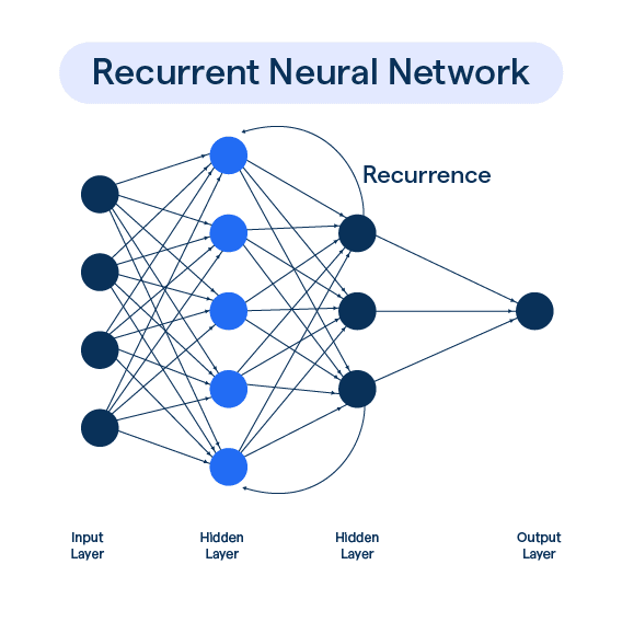
A Recurrent Neural Network (RNN) is uniquely designed for sequential data like time series. Its architecture enables the network to capture temporal patterns and dependencies, making it well-suited for forecasting and modeling sequences such as stock prices, weather data, and sensor measurements.
Core Components of RNN Architecture
-
Input Layer
- Receives time-series data, typically as sequences: at each step , the network takes an input value (or vector) .
-
Recurrent Hidden Layer(s)
- The heart of an RNN. Each neuron in this layer not only receives the current input but also the hidden state from the previous time step ().
- This structure lets the network retain and "remember" information across the sequence.
- Variants like LSTM and GRU cells are often used to solve standard RNNs' problems with long-term dependencies.
-
Output Layer
- Produces the prediction for each time step (can be one output for the whole sequence, or per step). For example, to predict the next value in a sequence, the output layer receives the hidden state and transforms it into a forecasted value.
Data Flow in an RNN (For a Sequence of Length T)
At each time step :
- Input: Receives
- Hidden State Update: Combines the input and previous hidden state to compute the new :
Where:
- is a nonlinear activation function (often tanh or ReLU)
- are weight matrices
- is bias
- Output: Optionally, each step may also produce an output .
Why RNNs Excel at Time-Series Modeling
- Sequential Memory: The recurrent structure lets RNNs learn relationships that depend on previous time steps, such as trends, seasonality, and patterns in time series.
- Flexible Inputs: RNNs handle variable-length input sequences, making them ideal for real-world time-series data.
- Extendable: Variants like LSTM and GRU enable RNNs to capture long-term dependencies and mitigate vanishing/exploding gradients. Advanced architectures can also integrate attention mechanisms or hybrid with CNNs.
Real-World Example
Suppose you're modeling daily sales: each day's sales plus the previous days' hidden state are used by the RNN to predict the next day's sales. The RNN 'remembers' recent sales patterns to produce better forecasts.
7) Compare RNN and LSTM architectures, highlighting the advantages of LSTM.
RNN vs LSTM: Architecture Comparison and LSTM Advantages
Basic RNN Architecture
- Structure: RNNs process sequential data by looping information (hidden state) from one step to the next. Each step takes the current input and previous hidden state to compute a new hidden state and output.
- Strengths: Good for short-term dependencies and quick pattern recognition.
- Limitations: Struggle with preserving information over long sequences due to the vanishing gradient problem—gradients become too small to update weights, so learning long-term patterns fails.
LSTM (Long Short-Term Memory) Architecture
- Structure: LSTMs are a special type of RNN designed to remember information over much longer sequences. Each LSTM cell includes:
- Memory Cell: Maintains information over many steps.
- Input Gate: Controls which new information enters the memory.
- Forget Gate: Controls which old information should be removed.
- Output Gate: Decides what part of the cell memory moves to the output.
- Strengths: The gating mechanisms allow LSTMs to retain important information and forget irrelevant details, thus capturing long-term dependencies in data.
- Limitations: LSTMs are more complex (more parameters and computations) and thus can be slower to train and require more memory compared to basic RNNs.
Key Advantages of LSTM over RNN
- Remembers Long-Term Patterns: LSTMs can capture long-range dependencies better by mitigating the vanishing gradient problem; basic RNNs quickly "forget" earlier sequence data.
- Selective Memory: With input, forget, and output gates, LSTMs decide what to remember, update, and forget, allowing for better handling of noisy or irrelevant information.
- Better Real-World Performance: LSTMs outperform RNNs in tasks like language modeling, machine translation, and speech recognition, where context from many steps in the past is crucial.
Summary Table
| Feature | RNN | LSTM |
|---|---|---|
| Memory Mechanism | Simple hidden state | Cell state plus input/forget/output gates |
| Long-term Dependency | Poor | Excellent |
| Vanishing Gradient Issue | Common | Rare (well-mitigated) |
| Complexity/Parameters | Fewer, simpler | More, higher memory/computation |
| Typical Use-Cases | Short-sequence modeling | Language, translation, time-series |
8) Explain the working principle of an autoencoder for unsupervised learning.
Working Principle of an Autoencoder for Unsupervised Learning
An autoencoder is a type of neural network designed to learn efficient representations of data in an unsupervised manner—meaning it does not use labeled outputs during training. Here is how it works step by step:
1. Architecture Overview
Autoencoders consist of three main parts:
- Encoder: Compresses the input data into a reduced, lower-dimensional representation (latent space or bottleneck). This step captures only the most important features and removes redundancy or noise.
- Bottleneck (Latent Space): The narrowest part of the network, storing the compact representation. Encoding data here forces the network to focus on essential features.
- Decoder: Reconstructs the original data from this compressed form, expanding it back to the original size and structure.
2. Training Process
- The input is first passed through the encoder, yielding the compressed (latent) code.
- The decoder then uses this code to reconstruct the input.
- The network is trained to minimize the reconstruction error—the difference between the original input and the reconstructed output (often using Mean Squared Error).
- Weights of both encoder and decoder are updated so that the autoencoder produces reconstructions as close as possible to the original data.
3. Key Points
- Unsupervised Learning: Autoencoders don’t require labeled data; they “supervise” themselves by trying to match their output to their own input.
- Feature Extraction & Dimensionality Reduction: By learning to faithfully compress and reconstruct inputs, autoencoders extract meaningful and useful features—even from noisy or redundant data.
4. Applications
- Data denoising, anomaly detection, dimensionality reduction, and as a pretraining step for deep learning tasks.
Quick Recap: You feed data in, the encoder compresses it, the decoder reconstructs it, and the network learns by minimizing the error between input and output—all without ever needing labeled outputs.
9) Differentiate between a standard autoencoder and a convolutional autoencoder.
Standard Autoencoder vs. Convolutional Autoencoder: Key Differences
Standard (Feedforward) Autoencoder
- Architecture: Uses fully connected (dense) layers in both encoder and decoder.
- Input Type: Works with flat (vectorized) data like tabular features, or reshaped images as 1D vectors.
- Feature Learning: Learns compressed representations by transforming the entire input space; does not explicitly capture spatial or local patterns—spatial structure in images may be lost.
- Typical Use Cases: Dimensionality reduction, anomaly detection on tabular data, and when global feature compression is enough.
Convolutional Autoencoder (CAE)
- Architecture: Uses convolutional layers in the encoder to extract spatial features and deconvolutional (upsampling) layers in the decoder for reconstruction.
- Input Type: Designed for image, video, or any grid-like data with spatial locality (e.g., 2D images, 3D volumes); input is kept in its original spatial shape (height x width x channels).
- Feature Learning: Excels at capturing local spatial features (edges, textures, patterns). By sliding filters over images, it learns efficient representations directly from pixel neighborhoods.
- Typical Use Cases: Image denoising, inpainting, super-resolution, and feature extraction for computer vision tasks.
Summary Table
| Feature | Standard Autoencoder | Convolutional Autoencoder |
|---|---|---|
| Layers | Fully connected (dense) | Convolutional & deconvolutional |
| Input Format | Flattened vectors | Images/grid data (preserve 2D/3D) |
| Spatial Info | Not preserved | Preserved & exploited |
| Best For | Generic, non-spatial data | Image and spatial data |
In short: CAEs are specialized autoencoders that use convolution to better process and reconstruct data with spatial structure, like images, while standard autoencoders use dense layers and are less suited for such tasks.
10) How does deep learning handle training with unlabeled data? Explain with an example.
How Deep Learning Handles Training with Unlabeled Data
Deep learning can effectively learn from unlabeled data using techniques from unsupervised learning. Unlike supervised learning, where models learn by mapping inputs to provided labels, unsupervised deep learning finds patterns, structures, and features in data without any explicit labels or target outputs.
Common Approaches in Deep Learning for Unlabeled Data
-
Clustering: Deep models (like neural networks) can be used to group similar data points into clusters (e.g., images with similar features), revealing hidden patterns or categories. For example, deep clustering can segment customers by behavior, or group images by visual similarity.
-
Autoencoders: An autoencoder is a type of neural network that learns to compress (encode) data into a smaller "latent space" and then reconstruct (decode) it back to the original form. During training, it never sees labels, only the input data itself. The network learns to preserve essential features, which can then be used for anomaly detection, noise reduction, or as learned features for other models.
Example: Given a large set of unlabeled handwritten digit images, an autoencoder learns to represent each image as a compact code by recreating the original input from this code. If you visualize codes for all images, you may see clusters corresponding to different digit types—without the model ever "knowing" what a digit is!
-
Generative Models (e.g., GANs): Networks like Generative Adversarial Networks (GANs) learn to generate new examples that resemble the original dataset. These models can reveal the underlying structure of the data and are widely used for synthetic data creation and augmentation.
Why Is This Useful?
- Pattern Discovery: Unlabeled data is much more plentiful and cheaper to collect than labeled data. Deep learning can extract useful features, spot anomalies, and reveal hidden groupings automatically.
- Foundation for Downstream Tasks: After unsupervised training, the learned features or representations can be used to improve supervised learning, such as through pre-training or transfer learning. For example, features from an autoencoder trained on unlabeled medical images can boost diagnostic accuracy once a smaller set of labeled images becomes available.
Real-World Example
Suppose an online retailer has millions of customer reviews but no labels about the sentiment (positive/negative). A deep learning model (like an autoencoder or clustering network) can analyze these reviews, organizing them into groups based on patterns—such as grouping similar phrases, tones, or topics. Later, these groupings can help in sentiment analysis, topic modeling, or even targeted marketing, all starting from unlabeled data.
Quick Recap: Deep learning leverages unsupervised learning methods—like clustering, autoencoders, and generative models—to automatically uncover patterns, group similar items, or extract useful representations from raw unlabeled data.
11) For an input image of size 32×32×3, with a convolutional layer of 5×5 filter, stride 1, padding 0, compute the output feature map size.
Let's compute the output feature map size after applying a convolutional layer to an input image of size 32×32×3 using a 5×5 filter, stride 1, and padding 0 (no padding).
Formula for Output Size
For each spatial dimension (height or width):
Plugging in the values:
- Input size = 32
- Filter size = 5
- Stride = 1
- Padding = 0
So, for both height and width, the output will be 28.
For the depth (channels), the output depth depends on the number of filters used. If you use, for example, 1 filter, the output feature map will have a depth of 1; with N filters, depth is N.
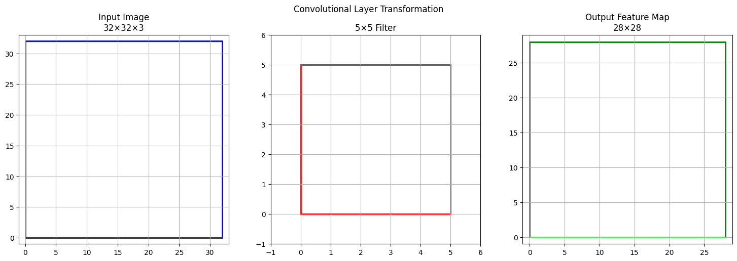
Final output feature map size (assuming 1 filter):
- 28 × 28 × 1
If your layer uses multiple filters, the output depth will be that number (e.g., for 16 filters: 28 × 28 × 16).
12) A CNN model uses 2 convolutional layers followed by max-pooling. Show the dimensionality changes for an input of 64×64×3 after each layer.
Let's walk step-by-step through the dimensionality changes when a 64×64×3 image passes through 2 convolutional layers (assuming common defaults: 3×3 filter, stride 1, padding 0) and then a max-pooling layer (assuming 2×2 pool size, stride 2).
Step 1: Input Layer
- Initial size: 64 × 64 × 3
Step 2: First Convolutional Layer
- Assumption: 3×3 filter, stride 1, padding 0 (valid)
- Output size formula:
(Input - Filter) / Stride + 1- (64 - 3)/1 + 1 = 62 → so 62 × 62
- Output depth: Depends on number of filters (let's use 8 for this example)
- After Conv1: 62 × 62 × 8
Step 3: Second Convolutional Layer
- Again, 3×3 filter, stride 1, padding 0
- (62 - 3)/1 + 1 = 60 → 60 × 60
- Use, say, 16 filters for this layer
- After Conv2: 60 × 60 × 16
Step 4: Max-Pooling Layer
- Typical pooling: 2×2 filter, stride 2
- (60 - 2)/2 + 1 = 30 → 30 × 30 × 16
Summary Table
| Layer | Output Size |
|---|---|
| Input | 64 × 64 × 3 |
| Conv1 | 62 × 62 × 8 |
| Conv2 | 60 × 60 × 16 |
| Max Pooling | 30 × 30 × 16 |
Note: Output channel numbers depend on the number of filters chosen; commonly, each convolutional layer increases the depth. You can plug in different filter, stride, or padding values to see how the dimensionality changes at each step.
13) Given a sequence [0.2, 0.4, 0.6], compute the hidden states of a simple RNN with weight = 0.5, initial hidden = 0, and sigmoid activation.
Let's compute the hidden states for a simple RNN given:
- Input sequence: [0.2, 0.4, 0.6]
- Weight: 0.5 (applies to both input and the hidden state)
- Initial hidden state: 0
- Activation: sigmoid
Formula Used
At each step :
with
Let's walk through each step:
Step 1 :
- Input
- Previous hidden
Step 2 :
- Input
- Previous hidden
Step 3 :
- Input
- Previous hidden
Final Hidden States
- h1 ≈ 0.525
- h2 ≈ 0.614
- h3 ≈ 0.647
Quick Check: Notice how the hidden state at each step carries forward information from both the current input and all previous steps. This is what gives RNNs their memory for handling sequences.